library(tidyverse)
library(ggplot2)
library(corrplot) # Various Scatter Plot
library(psych)    # Correlation Analysis
상관계수 (Correlation Coefficient)
다변수 확률변수 간의 상관관계를 숫자로 나타낸 것입니다. 보통 모상관계수는 \(\rho\), 표본상관계수는 \(r\)로 표기합니다. 표본상관계수 \(r\)의 부호는 상관관계의 방향을 나타내고, \(r\)의 크기는 상관관계의 정도를 나타냅니다.
| \(r\)의 부호 | 해석 |
|---|---|
| \(r\) > 0 | 양의 상관관계 |
| \(r\) < 0 | 음의 상관관계 |
| \(r\)의 절대값 | 해석 |
|---|---|
| 0.0 ~ 0.2 | 상관관계가 없다. |
| 0.2 ~ 0.4 | 약한 상관관계가 있다. |
| 0.4 ~ 0.6 | 보통의 상관관계가 있다. |
| 0.6 ~ 0.8 | 강하 상관관계가 있다. |
| 0.8 ~ 1.0 | 매우 강한 상관관계가 있다. |
R에서는 cor() 함수를 통해 상관계수를 구할 수 있는데, cor() 함수에 양적 자료를 할당하여 이를 구할 수 있습니다. 정규성 가정을 만족하는 경우 method = "pearson" 인자를 추가하여 피어슨 상관계수를 구할 수 있고, 정규성 가정을 만족하지 않거나 순위형 자료인 경우 method = "spearan" 혹은 method = "kendall" 인자를 추가합니다.
cor(cars$speed, cars$dist, method = "pearson")
## [1] 0.8068949
상관계수는 일반적으로 소수점 셋째자리까지 표현하는데, 위의 경우 상관계수가 약 0.807이라고 할 수 있습니다. 이는 speed와 dist 간에는 매우 강한 양의 상관관계가 있어보인다. 혹은 speed가 증가하면 dist도 증가하는 강한 경향을 보이고 있다.라고 해석할 수 있습니다.
상관계수행렬
다음과 같이 cor() 함수에 데이터셋을 할당하여 여러 변수 간의 상관계수를 구할 수도 있습니다. 이를 상관계수행렬이라고 합니다.
cor(attitude) # 상관계수행렬 출력
##               rating complaints privileges  learning    raises  critical
## rating     1.0000000  0.8254176  0.4261169 0.6236782 0.5901390 0.1564392
## complaints 0.8254176  1.0000000  0.5582882 0.5967358 0.6691975 0.1877143
## privileges 0.4261169  0.5582882  1.0000000 0.4933310 0.4454779 0.1472331
## learning   0.6236782  0.5967358  0.4933310 1.0000000 0.6403144 0.1159652
## raises     0.5901390  0.6691975  0.4454779 0.6403144 1.0000000 0.3768830
## critical   0.1564392  0.1877143  0.1472331 0.1159652 0.3768830 1.0000000
## advance    0.1550863  0.2245796  0.3432934 0.5316198 0.5741862 0.2833432
##              advance
## rating     0.1550863
## complaints 0.2245796
## privileges 0.3432934
## learning   0.5316198
## raises     0.5741862
## critical   0.2833432
## advance    1.0000000
round(cor(attitude), digits = 3)
##            rating complaints privileges learning raises critical advance
## rating      1.000      0.825      0.426    0.624  0.590    0.156   0.155
## complaints  0.825      1.000      0.558    0.597  0.669    0.188   0.225
## privileges  0.426      0.558      1.000    0.493  0.445    0.147   0.343
## learning    0.624      0.597      0.493    1.000  0.640    0.116   0.532
## raises      0.590      0.669      0.445    0.640  1.000    0.377   0.574
## critical    0.156      0.188      0.147    0.116  0.377    1.000   0.283
## advance     0.155      0.225      0.343    0.532  0.574    0.283   1.000
다른 방법으로는 psych 패키지의 corr.test() 함수를 사용하여 상관계수행렬을 구할 수도 있습니다.
psych::corr.test(attitude, method = "pearson")
## Call:psych::corr.test(x = attitude, method = "pearson")
## Correlation matrix
##            rating complaints privileges learning raises critical advance
## rating       1.00       0.83       0.43     0.62   0.59     0.16    0.16
## complaints   0.83       1.00       0.56     0.60   0.67     0.19    0.22
## privileges   0.43       0.56       1.00     0.49   0.45     0.15    0.34
## learning     0.62       0.60       0.49     1.00   0.64     0.12    0.53
## raises       0.59       0.67       0.45     0.64   1.00     0.38    0.57
## critical     0.16       0.19       0.15     0.12   0.38     1.00    0.28
## advance      0.16       0.22       0.34     0.53   0.57     0.28    1.00
## Sample Size
## [1] 30
## Probability values (Entries above the diagonal are adjusted for multiple tests.)
##            rating complaints privileges learning raises critical advance
## rating       0.00       0.00       0.19     0.00   0.01     1.00    1.00
## complaints   0.00       0.00       0.02     0.01   0.00     1.00    1.00
## privileges   0.02       0.00       0.00     0.07   0.15     1.00    0.51
## learning     0.00       0.00       0.01     0.00   0.00     1.00    0.03
## raises       0.00       0.00       0.01     0.00   0.00     0.36    0.01
## critical     0.41       0.32       0.44     0.54   0.04     0.00    0.90
## advance      0.41       0.23       0.06     0.00   0.00     0.13    0.00
##
##  To see confidence intervals of the correlations, print with the short=FALSE option
상관분석 (Correlation Analysis)
상관분석은 두개의 양적 자료 간에 상관관계가 있는지를 통계적으로 분석하는 방법입니다. 상관관계는 직선의 관계 즉 선형의 관계를 말합니다.이때 상관관계는 원인과 결과의 관계는 아닌데, 이러한 원인과 결과의 관계는 인과관계라고 합니다.
예제
attitude 데이터셋의 complaints와 rating 간에 상관관계가 있는지 분석하고자 합니다.
- 가설 설정
- 귀무가설 : complaints와 rating 간에는 관련성이 없다.
- 대립가설 : complaints와 rating 간에는 관련성이 있다.
- 정규성 검정
attitude %>%
  dplyr::select(complaints, rating) %>%
  purrr::map(shapiro.test)
## $complaints
##
##  Shapiro-Wilk normality test
##
## data:  .x[[i]]
## W = 0.97045, p-value = 0.5516
##
##
## $rating
##
##  Shapiro-Wilk normality test
##
## data:  .x[[i]]
## W = 0.9567, p-value = 0.2545
complaints와 rating 모두 정규성 가정을 만족합니다. 따라서 Pearson 상관분석을 실시합니다.
- Pearson 상관분석
cor.test(attitude$complaints, attitude$rating, method = "pearson")
##
##  Pearson's product-moment correlation
##
## data:  attitude$complaints and attitude$rating
## t = 7.737, df = 28, p-value = 1.988e-08
## alternative hypothesis: true correlation is not equal to 0
## 95 percent confidence interval:
##  0.6620128 0.9139139
## sample estimates:
##       cor
## 0.8254176
유의수준 0.05에서 유의확률이 0.000이므로 귀무가설을 기각합니다. 즉 complaints와 rating 간에는 통계적으로 유의한, 매우 강한 양의 상관관계(cor = 825)가 있는 것으로 나타납니다.
예제
cars 데이터셋의 speed와 dist 간에 상관관계가 있는지 분석하고자 합니다.
- 가설 설정
- 귀무가설 : speed와 dist 간에는 상관관계가 없다.
- 대립가설 : speed와 dist 간에는 상관관계가 있다.(관련성이 있다.)
- 정규성 검정
cars %>%
  purrr::map(shapiro.test)
## $speed
##
##  Shapiro-Wilk normality test
##
## data:  .x[[i]]
## W = 0.97765, p-value = 0.4576
##
##
## $dist
##
##  Shapiro-Wilk normality test
##
## data:  .x[[i]]
## W = 0.95144, p-value = 0.0391
speed는 정규성 가정을 만족하지만, dist는 정규성 가정을 만족하지 않습니다. 따라서 Spearman 혹은 Kendall 상관분석을 실시합니다.
- Spearman 상관분석 or Kendall 상관분석
cor.test(cars$speed, cars$dist, method = "spearman")
## Warning in cor.test.default(cars$speed, cars$dist, method = "spearman"): Cannot
## compute exact p-value with ties
##
##  Spearman's rank correlation rho
##
## data:  cars$speed and cars$dist
## S = 3532.8, p-value = 8.825e-14
## alternative hypothesis: true rho is not equal to 0
## sample estimates:
##       rho
## 0.8303568
cor.test(cars$speed, cars$dist, method = "kendall")
##
##  Kendall's rank correlation tau
##
## data:  cars$speed and cars$dist
## z = 6.6655, p-value = 2.638e-11
## alternative hypothesis: true tau is not equal to 0
## sample estimates:
##       tau
## 0.6689901
speed와 dist 간에 통계적으로 유의한 양의 상관관계가 있는 것으로 나타납니다.
산점도 (Scatter Plot)
plot()
plot(x = data$variable, y = data$variable) 함수를 통해 산점도를 그릴 수 있습니다.
plot() 함수에 첫번째로 할당된 양적 자료는 x축에, 두번째로 할당된 양적 자료는 y축에 표현됩니다. 더 중요하게 생각하는 양적 자료를 y축에 표현하는 것이 일반적입니다.
plot(cars$speed, cars$dist, col = "red", pch = 15, cex = 0.5)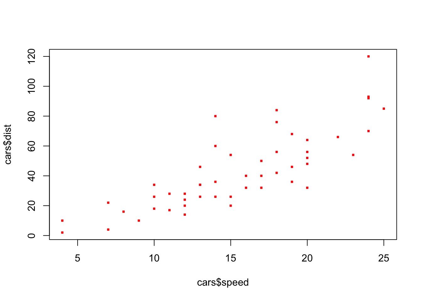
ggplot2
cars %>%
  ggplot2::ggplot(mapping = aes(x = speed, y = dist)) +
  ggplot2::geom_point(color = "red")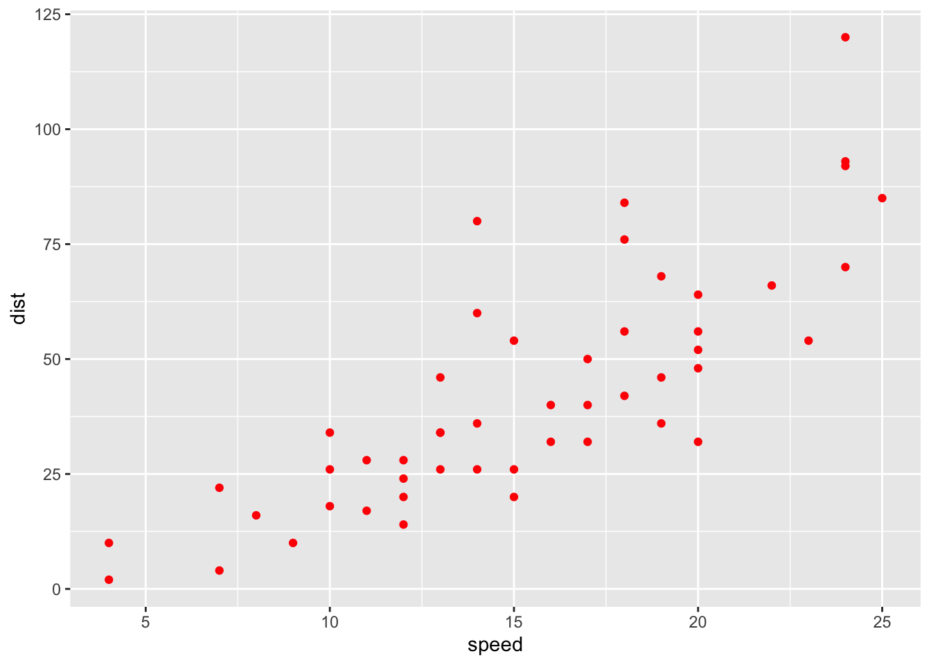
diamonds %>%
  dplyr::sample_frac(size = 0.01) %>%
  ggplot2::ggplot(mapping = aes(x = carat, y = price)) +
  ggplot2::geom_point(aes(color = cut))
diamonds %>%
  dplyr::sample_frac(size = 0.01) %>%
  ggplot2::ggplot(mapping = aes(x = carat, y = price)) +
  ggplot2::geom_point() +
  ggplot2::facet_wrap(~cut)
diamonds %>%
  dplyr::sample_frac(size = 0.01) %>%
  ggplot2::ggplot(mapping = aes(x = carat, y = price)) +
  ggplot2::geom_point() +
  ggplot2::geom_jitter() # 겹쳐진 점들을 조정
산점행렬도 (Scatter Plot Matrix ; SPM)
산점행렬도는 하나의 그래프에 여러개의 산점도를 작성하는 것을 말합니다. R에서는 plot() 함수와 corrplot() 함수를 활용하여 산점행렬도를 그릴 수 있습니다.
plot()
plot() 함수를 사용할 때에는 해당 데이터셋에 양적 자료만 있어야 합니다.
plot(attitude)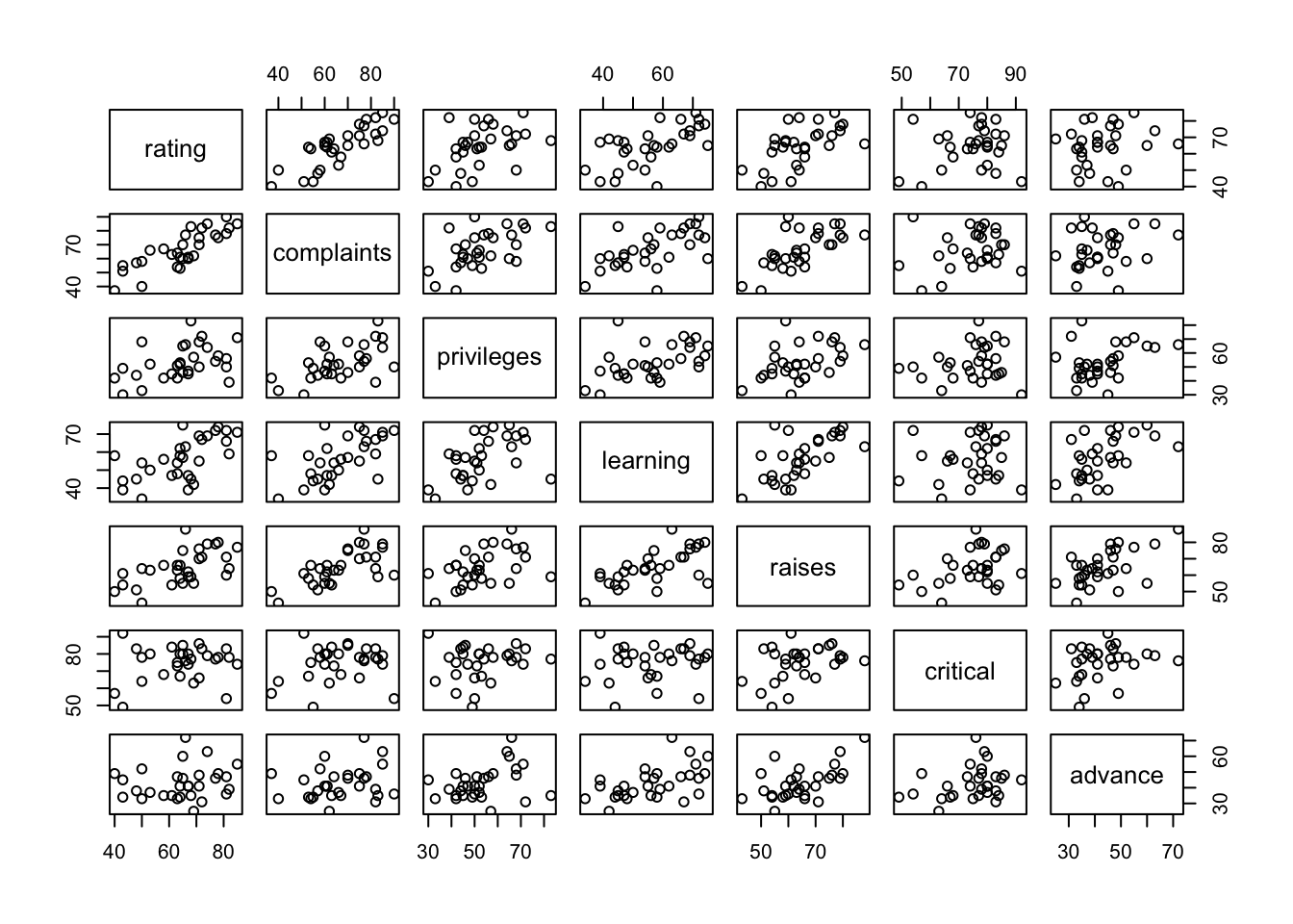
diamonds 데이터셋에서 1%의 표본을 추출하고 이 데이터 중에서 수치형 데이터에 대한 산점행렬도를 작성하면 다음과 같습니다.
diamonds %>%
  dplyr::sample_frac(size = 0.01) %>%
  purrr::keep(is.numeric) %>%
  plot()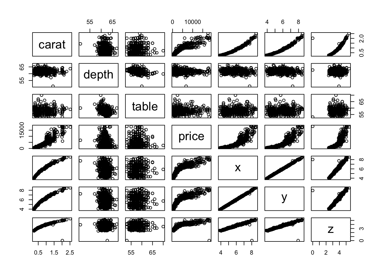
corrplot()
corrplot 패키지의 corrplot() 함수를 통해 산점행렬도를 그릴 수 있습니다. 이때 주의해야 할 점은 plot() 함수에서는 데이터셋을 할당한 반면 corrplot() 함수에서는 아래와 같이 상관계수행렬을 할당해야 합니다.
corrplot(cor(mtcars))
corrplot() 함수로 그린 산점행렬도에서는 양의 상관관계가 파란색으로, 음의 상관관계가 빨간색으로 표현됩니다. 색의 강도와 원의 크기는 상관계수에 비례합니다.
corrplot() 함수는 그래프를 다양하게 표현할 수 있도록 여러 인자를 지원해주고 있습니다. 자세히 살펴보면 다음과 같습니다.
| argument | value | description |
|---|---|---|
| method | “circle” (default) | - |
| method | “square” | - |
| method | “ellipse” | - |
| method | “number” | - |
| method | “shade” | - |
| method | “color” | - |
| method | “pie” | - |
| type | “full” (default) | display full correlation matrix |
| type | “upper” | display upper triangular of the correlation matrix |
| type | “lower” | display lower triangular of the correlation matrix |
이제 코드를 통해 하나씩 살펴보겠습니다.
method = "ellipse"는 그래프에서 상관관계를 타원으로 표현해줍니다.
corrplot(cor(mtcars), method = "ellipse")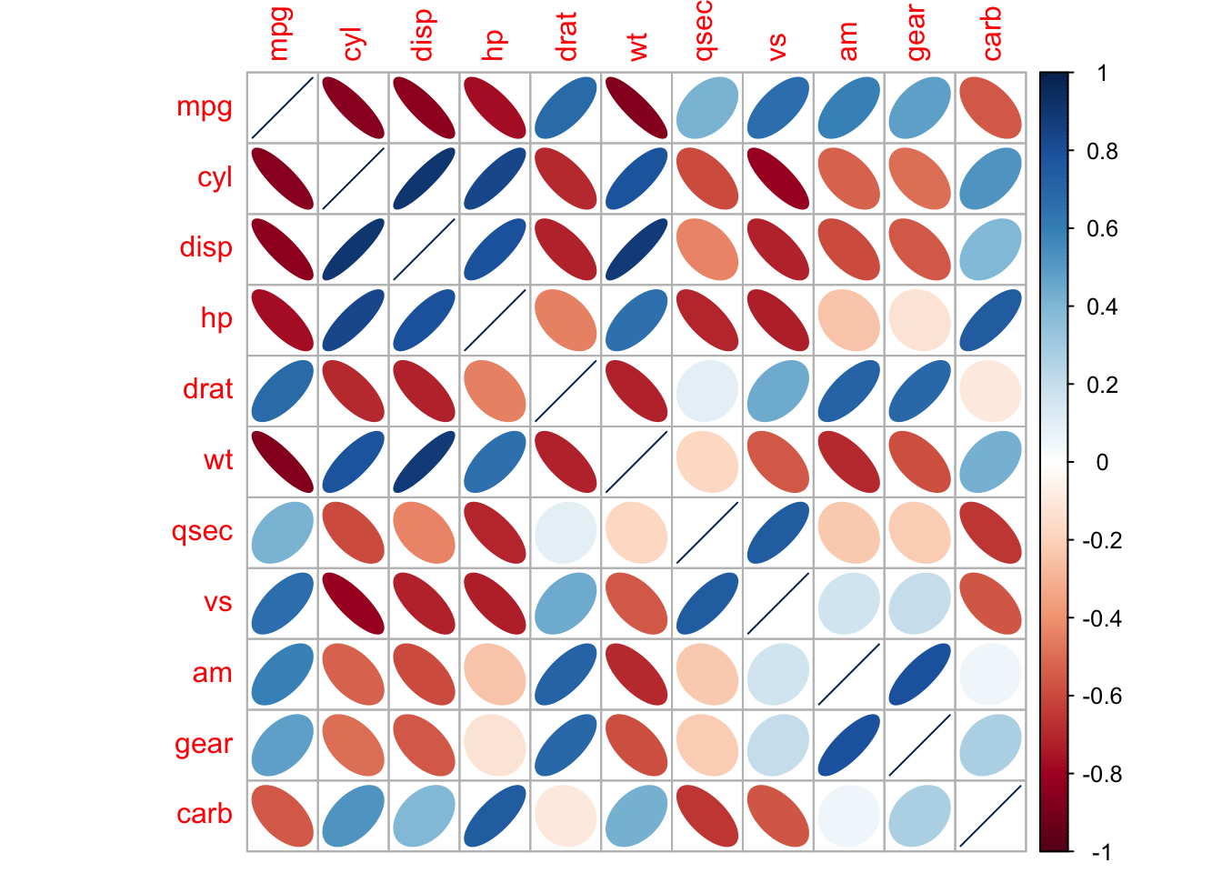
method = "number" 인자는 그래프에서 상관관계를 상관계수로 표현해줍니다.
corrplot(cor(mtcars), method = "number")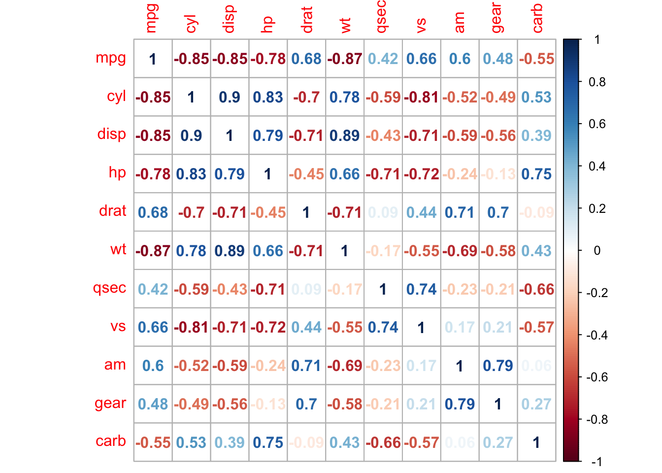
method = "color" 인자는 그래프에서 상관관계를 색깔로 칠해 표현해줍니다.
corrplot(cor(mtcars), method = "color")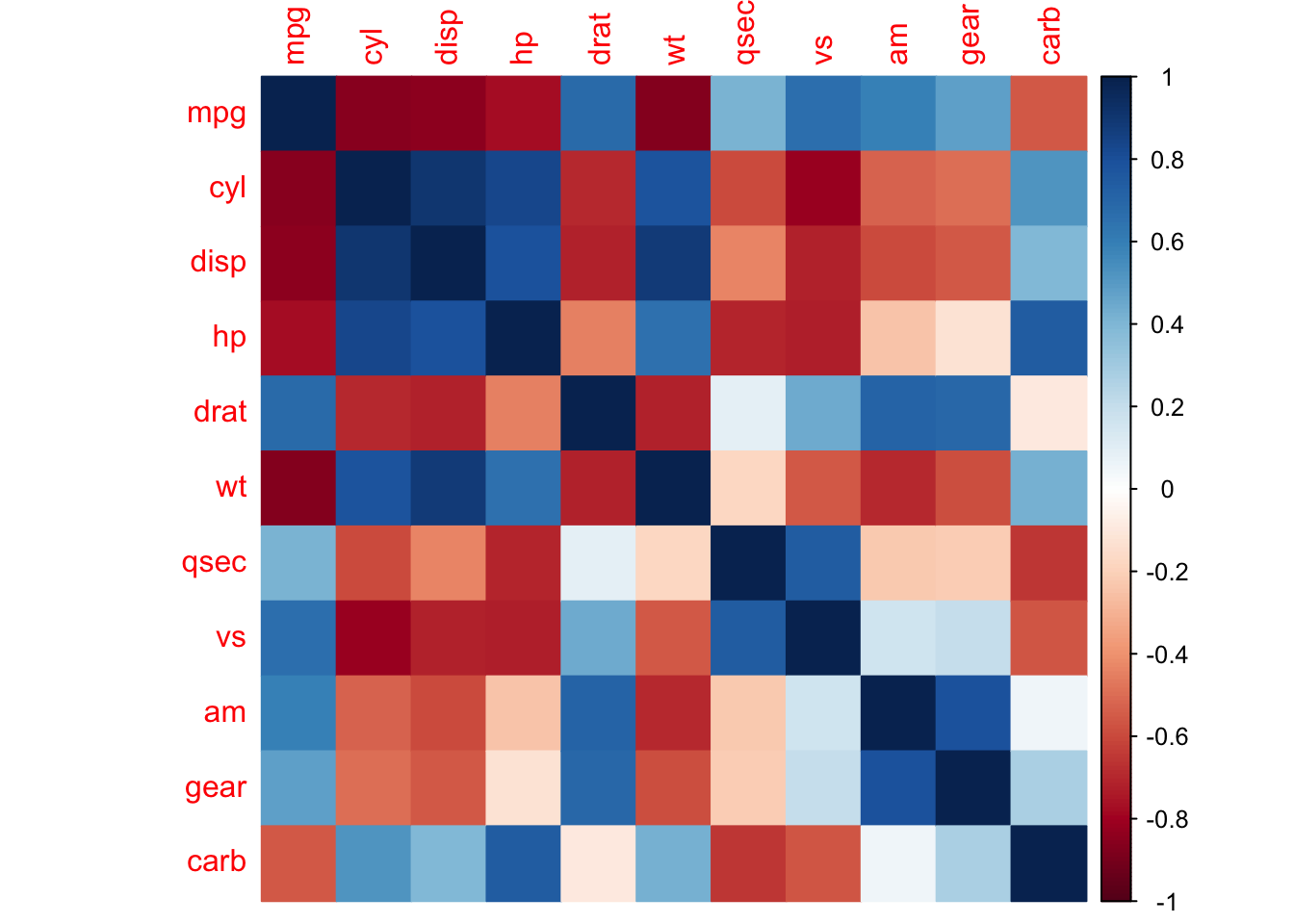
type = "upper" 인자는 그래프를 위쪽만 보여줍니다.
corrplot(cor(mtcars), type = "upper")